Neural Architectures

Convolutional Architecture

Convolution

Convolution is a mathematical operation that combines two functions to produce a third function:

$$\begin{equation} (f*g)(t):=\int_{-\infty}^{\infty} f(\tau)g(t-\tau)d\tau \end{equation}$$

Given $\boldsymbol{a}$ and $\boldsymbol{b}$, then: $(\boldsymbol{a}*\boldsymbol{b})_n=\sum\limits_{\substack{i,j\\i+j=n}}a_i\cdot{b_j}$, e.g. $(1,2,3)*(4,5,6)=(4,13,28,27,18)_{0\dots{4}}$. 上述计算可以转换为多项式相乘的形式:

$$\begin{split} A(x)&=\sum\limits_{i=0}^{M-1}a_i\cdot{x^i} \\ B(x)&=\sum\limits_{i=0}^{N-1}b_i\cdot{x^i} \\ C(x)&=A(x)\cdot{B(x)} \\ C(x)&=\sum\limits_{i=0}^{M+N-2}c_i\cdot{x^i} \\ c_i&=\sum\limits_{j=0}^{i}a_j\cdot{b_{i-j}} \end{split}$$

可以运用快速傅里叶变换 (FFT) 以 $O(N\log N)$ 的时间复杂度求解 $c_i$ 的值, 从而实现快速卷积运算.

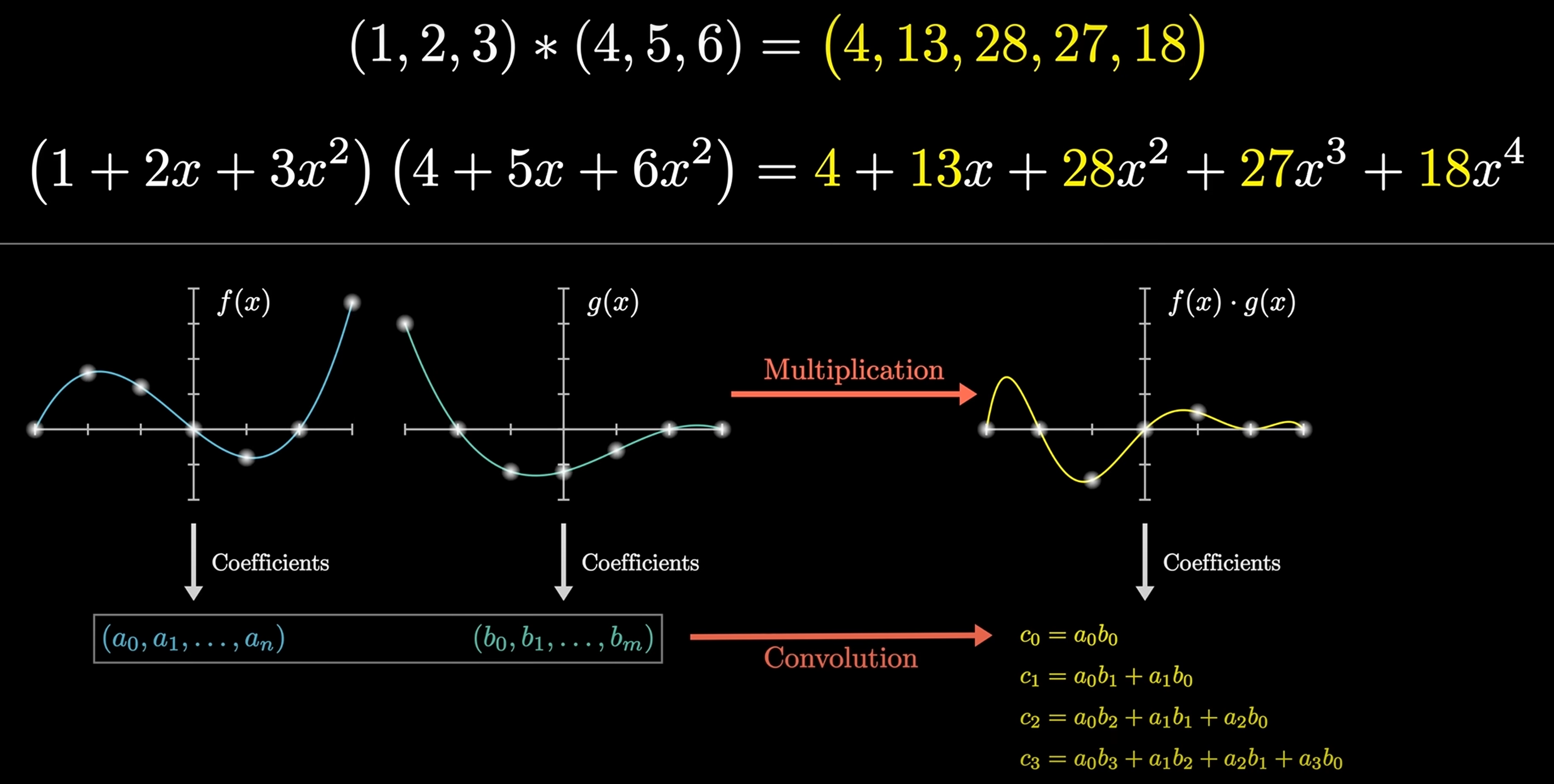
For matrix:

$$B(i,j)=\sum\limits_{m=0}^{M_k-1}\sum\limits_{n=0}^{N_k-1} K(m, n) A(i-m, j-n)$$

Convolutional Neural Networks

CNNs are a class of deep neural networks, most commonly applied to analyzing visual imagery. They are also known as ConvNets:

• Input Layer (输入层): raw pixel values of an image.
• Hidden Layers (隐藏层):
  • Convolutional Layer (卷积层): find patterns in regions of the input, and passing the results to the next layer.
  • Pooling Layer (池化层): down-samples the input representation, reducing its dimensionality.
  • Fully Connected Layer (全连接层): compute the class scores, resulting in a volume of size $1\times1\times{n}$, where each of the $n$ numbers represents a class.
• Output Layer (输出层): class scores.

# Load the data and split it between train and test sets
(x_train, y_train), (x_test, y_test) = keras.datasets.mnist.load_data()

# Scale images to the [0, 1] range
x_train = x_train.astype("float32") / 255
x_test = x_test.astype("float32") / 255
# Make sure images have shape (28, 28, 1)
x_train = np.expand_dims(x_train, -1)
x_test = np.expand_dims(x_test, -1)
print("x_train shape:", x_train.shape)
print("y_train shape:", y_train.shape)
print(x_train.shape[0], "train samples")
print(x_test.shape[0], "test samples")

# Model parameters
num_classes = 10
input_shape = (28, 28, 1)

model = keras.Sequential(
    [
        keras.layers.Input(shape=input_shape),
        keras.layers.Conv2D(64, kernel_size=(3, 3), activation="relu"),
        keras.layers.Conv2D(64, kernel_size=(3, 3), activation="relu"),
        keras.layers.MaxPooling2D(pool_size=(2, 2)),
        keras.layers.Conv2D(128, kernel_size=(3, 3), activation="relu"),
        keras.layers.Conv2D(128, kernel_size=(3, 3), activation="relu"),
        keras.layers.GlobalAveragePooling2D(),
        keras.layers.Dropout(0.5),
        keras.layers.Dense(num_classes, activation="softmax"),
    ]
)

model.compile(
    loss=keras.losses.SparseCategoricalCrossEntropy(),
    optimizer=keras.optimizers.Adam(learning_rate=1e-3),
    metrics=[
        keras.metrics.SparseCategoricalAccuracy(name="acc"),
    ],
)

# Train
batch_size = 128
epochs = 20

callbacks = [
    keras.callbacks.ModelCheckpoint(filepath="model_at_epoch_{epoch}.keras"),
    keras.callbacks.EarlyStopping(monitor="val_loss", patience=2),
]

model.fit(
    x_train,
    y_train,
    batch_size=batch_size,
    epochs=epochs,
    validation_split=0.15,
    callbacks=callbacks,
)
score = model.evaluate(x_test, y_test, verbose=0)

# Save model
model.save("final_model.keras")

# Predict
predictions = model.predict(x_test)

Convolutional Layer

Convolutional Layer is the first layer to extract features from an input image. The layer's parameters consist of a set of learnable filters (or kernels), which have a small receptive field but extend through full depth of input volume.

Pooling Layer

Pooling Layer is used to reduce the spatial dimensions of the input volume. It helps to reduce the amount of parameters and computation in the network, and hence to also control overfitting.

Fully Connected Layer

Fully Connected Layer is a traditional Multilayer Perceptron (MLP) layer. It is used to compute the class scores, resulting in a volume of size $1\times1\times{n}$, where each of the $n$ numbers represents a class.

Spatial Transformer Networks

传统的池化方式 (Max Pooling/Average Pooling) 所带来卷积网络的位移不变性和旋转不变性只是局部的和固定的, 且池化并不擅长处理其它形式的仿射变换.

Spatial transformer networks (STNs) allow a neural network to learn how to perform spatial transformations on the input image in order to enhance the geometric invariance of the model. STNs 可以学习一种变换, 这种变换可以将仿射变换后的图像进行矫正, 保证 CNNs 在输入图像发生变换时, 仍然能够保持稳定的输出 (可视为总是输入未变换的图像).

Recurrent Architecture

Recurrent Neural Networks

循环神经网络 (RNNs) 是一种具有循环结构的神经网络, 可以处理序列数据, 例如时间序列数据, 自然语言文本等.

当序列数据输入到 RNNs 中时, 每个时间步都会产生一个输出, 并将隐藏状态 (Hidden State) 传递到下一个时间步. 因此, 当改变输入序列的顺序时, RNNs 会产生不同的输出 (Changing sequence order will change output).

$$\begin{equation} \begin{split} h_t&=\sigma(W_hh_{t-1}+W_ix_t+b_h) \\ y_t&=\sigma(W_oh_t+b_y) \end{split} \end{equation}$$

Long Short-Term Memory

长短期记忆网络 (LSTM) 是一种特殊的 RNN, 通过引入门控机制 (Gate Mechanism) 来控制信息的流动, 解决了长序列训练过程中的梯度消失和梯度爆炸问题.

$$\begin{equation} \begin{split} f_t&=\sigma(W_f\cdot[h_{t-1},x_t]+b_f) \\ i_t&=\sigma(W_i\cdot[h_{t-1},x_t]+b_i) \\ \tilde{C}_t&=\tanh(W_C\cdot[h_{t-1},x_t]+b_C) \\ C_t&=f_t*{C_{t-1}}+i_t*\tilde{C}_t \\ o_t&=\sigma(W_o\cdot[h_{t-1},x_t]+b_o) \\ h_t&=o_t*\tanh(C_t) \\ y_t&=\sigma(W_yh_t+b_y) \end{split} \end{equation}$$

Residual Architecture

ResNet 通过残差学习解决了深度网络的退化问题 (深度网络的训练问题), 最短的路, 决定容易优化的程度: 残差连接 (Residual Connection) 可以认为层数是 0. 最长的路, 决定深度网络的能力: 解决了深度网络的训练问题后, 可以做到更深的网络 (100+).

ResNet 通过引入残差连接, 允许网络学习残差映射而不是原始映射. 残差映射就是目标层与它的前面某层之间的差异 $\mathcal{F}(\mathrm{x}):=\mathcal{H}(\mathrm{x})-\mathrm{x}$. 如果输入和输出之间的差异很小, 那么残差网络只需要学习这些微小的差异即可. 这种学习通常比学习原始的复杂映射要简单得多.

$$\begin{equation} \begin{split} \mathrm{y}&=\mathcal{F}(\mathrm{x}, W_i)+W_s\mathrm{x} \\ &=\mathcal{F}(\mathrm{x})+\mathrm{x} \\ &=\mathcal{H}(\mathrm{x})-\mathrm{x}+\mathrm{x} \\ &=\mathcal{H}(\mathrm{x}) \end{split} \end{equation}$$

从深层网络角度来讲, 不同的层学习的速度差异很大, 表现为网络中靠近输出的层学习的情况很好, 靠近输入的层学习的很慢, 有时甚至训练了很久, 前几层的权值和刚开始随机初始化的值差不多 (无法收敛). 因此, 梯度消失或梯度爆炸的根本原因在于反向传播训练法则, 本质在于方法问题. ResNet 通过残差连接保持梯度传播, 使得网络的训练更加容易:

$$\begin{equation} \frac{\theta{f(g(x))+g(x)}}{\theta{x}}= \frac{\theta{f(g(x))}}{\theta{g(x)}}\cdot{\frac{\theta{g(x)}}{\theta{x}}}+\frac{\theta{g(x)}}{\theta{x}} \end{equation}$$