Transformer
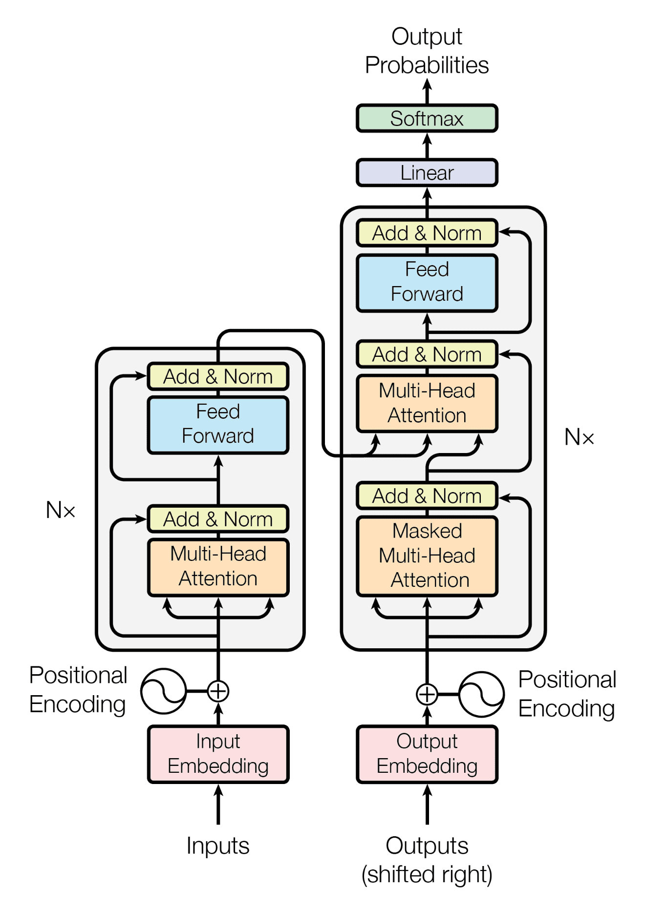
- Self-attention only: comparing to Recurrent Neural Networks (RNNs), no recurrent layers, allows for more parallelization.
- Multi-headed attention: consistent with Convolutional Neural Networks (CNNs), multiple output channels.
Self-Attention Mechanism
In layman's terms, a self-attention module takes in n inputs and returns n outputs:
- Self: allows the inputs to interact with each other
- Attention: find out who they should pay more attention to.
- The outputs are aggregates of these interactions and attention scores.
The illustrations are divided into the following steps:
- Prepare inputs.
- Weights initialization (Constant/Random/Xavier/Kaiming Initialization).
- Derive query, key and value.
- Calculate attention scores for input.
- Calculate softmax.
- Multiply scores with values.
- Sum weighted values to get output.
Weights for query, key and value (these weights are usually small numbers, initialized randomly using an appropriate random distribution like Gaussian, Xavier and Kaiming distributions):
Derive query, key and value:
Calculate attention scores for input:
为行向量分别与自己和其他两个行向量做内积 (点乘), 向量的内积表征两个向量的夹角 (), 表征一个向量在另一个向量上的投影, 投影的值大, 说明两个向量相关度高 (Relevance/Similarity).
Softmaxed attention scores :
softmax function:
其中, 为温度参数 (Temperature Parameter),
用于控制 softmax 函数的输出分布的陡峭程度:
- 时,
softmax函数退化为标准形式. - 时,
softmax函数输出分布更加平缓. - 时,
softmax函数输出分布更加陡峭. - 时,
softmax函数退化为argmax函数, 输出分布中只有一个元素为 1, 其他元素为 0.
矩阵 中每一个元素除以 后, 方差变为 1. 这使得 的分布"陡峭"程度与 解耦, 从而使得训练过程中梯度值保持稳定.
Alignment vectors (yellow vectors) addition to output:
Repeat for every input:
Calculate by matrix multiplication:
Self-attention 中的 思想,
另一个层面是想要构建一个具有全局语义 (Context) 整合功能的数据库,
使得 Context Size 内的每个元素都能够看到其他元素的信息,
从而能够更好地进行决策.
import torch
from torch.nn.functional import softmax

# 1. Prepare inputs
x = [
    [1, 0, 1, 0],  # Input 1
    [0, 2, 0, 2],  # Input 2
    [1, 1, 1, 1],  # Input 3
]
x = torch.tensor(x, dtype=torch.float32)

# 2. Weights initialization
w_query = [
    [1, 0, 1],
    [1, 0, 0],
    [0, 0, 1],
    [0, 1, 1],
]
w_key = [
    [0, 0, 1],
    [1, 1, 0],
    [0, 1, 0],
    [1, 1, 0],
]
w_value = [
    [0, 2, 0],
    [0, 3, 0],
    [1, 0, 3],
    [1, 1, 0],
]
w_query = torch.tensor(w_query, dtype=torch.float32)
w_key = torch.tensor(w_key, dtype=torch.float32)
w_value = torch.tensor(w_value, dtype=torch.float32)

# 3. Derive query, key and value
queries = x @ w_query
keys = x @ w_key
values = x @ w_value

# 4. Calculate attention scores
attn_scores = queries @ keys.T

# 5. Calculate softmax
attn_scores_softmax = softmax(attn_scores, dim=-1)
# tensor([[6.3379e-02, 4.6831e-01, 4.6831e-01],
#         [6.0337e-06, 9.8201e-01, 1.7986e-02],
#         [2.9539e-04, 8.8054e-01, 1.1917e-01]])
# For readability, approximate the above as follows
attn_scores_softmax = [
    [0.0, 0.5, 0.5],
    [0.0, 1.0, 0.0],
    [0.0, 0.9, 0.1],
]
attn_scores_softmax = torch.tensor(attn_scores_softmax)

# 6. Multiply scores with values
weighted_values = values[:, None] * attn_scores_softmax.T[:, :, None]

# 7. Sum weighted values
outputs = weighted_values.sum(dim=0)

print(outputs)
# tensor([[2.0000, 7.0000, 1.5000],
#         [2.0000, 8.0000, 0.0000],
#         [2.0000, 7.8000, 0.3000]])
# tensor([[1.9366, 6.6831, 1.5951],
#         [2.0000, 7.9640, 0.0540],
#         [1.9997, 7.7599, 0.3584]])
自注意力机制能够直接建模序列中任意两个位置之间的关系, 进而有效捕获长程依赖关系, 具有更强的序列建模能力. 自注意力的计算过程对于基于硬件的并行优化 (GPU/TPU) 非常友好, 因此能够支持大规模参数的高效优化.
Multi-Head Attention Mechanism
Multiple output channels:
from math import sqrt
import torch
import torch.nn

class Self_Attention(nn.Module):
    # input : batch_size * seq_len * input_dim
    # q : batch_size * input_dim * dim_k
    # k : batch_size * input_dim * dim_k
    # v : batch_size * input_dim * dim_v
    def __init__(self, input_dim, dim_k, dim_v):
        super(Self_Attention, self).__init__()
        self.q = nn.Linear(input_dim, dim_k)
        self.k = nn.Linear(input_dim, dim_k)
        self.v = nn.Linear(input_dim, dim_v)
        self._norm_fact = 1 / sqrt(dim_k)

    def forward(self, x):
        Q = self.q(x)  # Q: batch_size * seq_len * dim_k
        K = self.k(x)  # K: batch_size * seq_len * dim_k
        V = self.v(x)  # V: batch_size * seq_len * dim_v

        # Q * K.T() # batch_size * seq_len * seq_len
        attention = nn.Softmax(dim=-1)(torch.bmm(Q, K.permute(0, 2, 1))) * self._norm_fact

        # Q * K.T() * V # batch_size * seq_len * dim_v
        output = torch.bmm(attention, V)

        return output

class Self_Attention_Multiple_Head(nn.Module):
    # input : batch_size * seq_len * input_dim
    # q : batch_size * input_dim * dim_k
    # k : batch_size * input_dim * dim_k
    # v : batch_size * input_dim * dim_v
    def __init__(self, input_dim, dim_k, dim_v, nums_head):
        super(Self_Attention_Multiple_Head, self).__init__()
        assert dim_k % nums_head == 0
        assert dim_v % nums_head == 0
        self.q = nn.Linear(input_dim, dim_k)
        self.k = nn.Linear(input_dim, dim_k)
        self.v = nn.Linear(input_dim, dim_v)

        self.nums_head = nums_head
        self.dim_k = dim_k
        self.dim_v = dim_v
        self._norm_fact = 1 / sqrt(dim_k)

    def forward(self, x):
        Q = self.q(x).reshape(-1, x.shape[0], x.shape[1], self.dim_k // self.nums_head)
        K = self.k(x).reshape(-1, x.shape[0], x.shape[1], self.dim_k // self.nums_head)
        V = self.v(x).reshape(-1, x.shape[0], x.shape[1], self.dim_v // self.nums_head)
        print(x.shape)
        print(Q.size())

        # Q * K.T() # batch_size * seq_len * seq_len
        attention = nn.Softmax(dim=-1)(torch.matmul(Q, K.permute(0, 1, 3, 2)))

        # Q * K.T() * V # batch_size * seq_len * dim_v
        output = torch.matmul(attention, V).reshape(x.shape[0], x.shape[1], -1)

        return output
Positional Encoding Mechanism
位置编码 使用正弦和余弦函数的 d 维向量编码方法, 用于在输入序列中表示每个单词的位置信息, 丰富了模型的输入数据, 为其提供位置信息 (把词序信号加到词向量上帮助模型学习这些信息):
- 唯一性 (Unique): 为每个时间步输出一个独一无二的编码.
- 一致性 (Consistent): 不同长度的句子之间, 任何两个时间步之间的距离保持一致.
- 泛化性 (Generalizable): 模型能毫不费力地泛化到更长的句子, 位置编码的值是有界的.
- 确定性 (Deterministic): 位置编码的值是确定性的.
编码函数使用正弦和余弦函数, 其频率沿着向量维度进行减少. 编码向量包含每个频率的正弦和余弦对, 以实现 和 的线性变换, 从而有效地表示相对位置.
For (where ), then
where
outcomes
KV Cache
Prompt caching
缓存的不是文本是思维状态, 本质是复用 KV 矩阵.